Yesterday we had Mother’s Day in Poland. Since my girlfriend and I are parents of our cute pug called Delta, we decided to help her with a gift for mommy. She decided to give her mother a curve. Delta wanted to learn how to make Wolfram|Alpha style person curves like this:

You can easily generate this by yourself by typing Barack Obama curve into Wolfram|Alpha. Ok, but she did something way better. She curved herself! Let’s compare the photo she used with her final work:

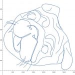
As you can see, her plot bears resemblance to the real picture. And this is not just a mere drawing, this is a parametric plot of an actual function! I will now guide you how to make such curves by yourself. Our discussion will be based on a blog post made by Michael Trott, Chief Scientist at Wolfram|Alpha. Micheal’s insights are more specific than what I will discuss, so please refer to his work for a more detailed explanation.
First, we have to define some functions that we will use later. Just copy this extreme chunk of code into your Mathematica and evaluate all cells:
[code language=”java” collapse=”true” title=”Click here to expand the code. Again, this is a code by Michael Trott. See Micheal’s blog if you have any questions on this.”]
fourierComponentData[pointList_, nMax_, op_] :=
Module[{\[CurlyEpsilon]=10^-3, \[Mu] = 2^14, M = 10000,s,
scale, \[CapitalDelta], L , nds, sMax, if, \[ScriptX]\[ScriptY]Function, X, Y, XFT, YFT,type},
(* prepare curve *)
scale = 1. Mean[Table[ Max[ fl/@ pointList] – Min[fl /@ pointList],{fl,{First, Last}}]];
\[CapitalDelta]=EuclideanDistance[First[pointList], Last[pointList]];
L=Which[op === “Closed”, type=”Closed”;
If[First[pointList]===Last[pointList],
pointList,Append[pointList, First[pointList]]],
op === “Open”,type=”Open”;pointList,
\[CapitalDelta]==0.,type=”Closed”; pointList,
\[CapitalDelta]/scale4];
nds = NDSolve[{s'[t]==Sqrt[\[ScriptX]\[ScriptY]Function'[t].\[ScriptX]\[ScriptY]Function'[t]], s[0]==0},s,
{t, 0, 1}, MaxSteps -> 10^5, PrecisionGoal -> 4];
(* total curve length *)
sMax= s[1]/.nds[[1]];
if=Interpolation[Table[{s[\[Sigma]]/.nds[[1]], \[Sigma]}, {\[Sigma],0, 1, 1/M}]];
X[t_Real] := BSplineFunction[L][Max[Min[1, if[(t +Pi)/(2Pi)sMax]] , 0]][[1]];
Y[t_Real] := BSplineFunction[L][Max[Min[1, if[(t +Pi)/(2Pi)sMax]] , 0]][[2]];
(* extract Fourier coefficients *)
{XFT, YFT} = Fourier[Table[#[N @ t], {t, -Pi+\[CurlyEpsilon], Pi – \[CurlyEpsilon], (2Pi-2\[CurlyEpsilon])/\[Mu]}]]& /@ {X, Y};
{type,2Pi/Sqrt[\[Mu]] *
((Transpose[Table[{Re[#], Im[#]}&[Exp[I k Pi] #[[k+1]]], {k, 0, nMax}]]& /@ {XFT, YFT}))} ]
Options[fourierComponents] = {“MaxOrder” -> 180, “OpenClose” -> 0.025};
fourierComponents[pointLists_,OptionsPattern[]] :=
Monitor[Table[fourierComponentData[pointLists[[k]],
If[Head[#]===List, #[[k]], #]&[ OptionValue[“MaxOrder”]],
If[Head[#]===List, #[[k]], #]&[ OptionValue[“OpenClose”]]],
{k, Length[pointLists]}],
Grid[{{Text[Style[“progress calculating Fourier coefficients”, Darker[Green, 0.66]]], ProgressIndicator[k/Length[pointLists]]} },
Alignment -> Left, Dividers -> Center]]/; Depth[pointLists] === 4
makeSegmentOrderManipulate[fCs_, orderList_, maxOrder_Integer: 60,
graphicsOptions_Rule …] :=
With[{nVars =
Table[ToExpression[“n” IntegerString[k]], {k, Length[fCs]}]},
Manipulate[
Module[{
highlightColor =
Directive[Thickness[0.01], Purple, Opacity[0.5]], tab,
curvesNew, pos, gr},
(* initialize variable curves *)
If[curves === {},
tab = Table[ ParametricPlot[Evaluate[
{Sum[
If[k == 0, 1/2, 1] fCs[[m, 2, 1, 1, k + 1]] Cos[k t] +
fCs[[m, 2, 1, 2, k + 1]] Sin[k t],
Evaluate[{k, 0, nVars[[m]]}],
Method -> “Procedural”],
Sum[If[k == 0, 1/2, 1] fCs[[m, 2, 2, 1, k + 1]] Cos[k t] +
fCs[[m, 2, 2, 2, k + 1]] Sin[k t],
Evaluate[{k, 0, nVars[[m]]}],
Method -> “Procedural”]}],
Evaluate[{t, If[fCs[[m, 1]] === “Closed”, -Pi, 0], Pi}],
MaxRecursion -> 3, PlotRange -> All,
(* highlight segment of clicked-in slider *)
PlotStyle -> Black, Frame -> True, Axes -> False,
FrameTicks -> None, PerformanceGoal -> “Quality”],
{m, Length[fCs]}] ;
curves = Cases[#, _Line, \[Infinity]] & /@ tab ];
(* position last changed slider value *)
pos = Flatten[
Position[ Abs[nVars – nVals], Except[0], {1}, Heads -> False]];
(* draw curve of slider moved *)
If[pos =!= {},
curvesNew = Table[Cases[
ParametricPlot[Evaluate[ With[{m = pos[[j]]},
{
Sum[If[k == 0, 1/2, 1] fCs[[m, 2, 1, 1, k + 1]] Cos[
k t] + fCs[[m, 2, 1, 2, k + 1]] Sin[k t],
Evaluate[{k, 0, nVars[[m]]}],
Method -> “Procedural”],
Sum[If[k == 0, 1/2, 1] fCs[[m, 2, 2, 1, k + 1]] Cos[
k t] + fCs[[m, 2, 2, 2, k + 1]] Sin[k t],
Evaluate[{k, 0, nVars[[m]]}],
Method -> “Procedural”]}]],
Evaluate[{t, If[fCs[[m, 1]] === “Closed”, -Pi, 0], Pi}],
MaxRecursion -> 3, PlotRange -> All,
Frame -> True, Axes -> False, FrameTicks -> None,
PerformanceGoal -> “Quality”], _Line, \[Infinity]],
{j, Length[pos]}];
(* highlight changed curve *)
Do[curves = MapAt[ curvesNew[[j]] &, curves, pos[[j]]], {j,
Length[pos]}]];
gr =
Graphics[{Black,
MapAt[{highlightColor, #} &,
If[cN === 0, curves ,
MapAt[{highlightColor, #} &, curves, cN]],
If[ControlActive[True, False], List /@ pos, {}]]},
ImageSize -> 360, graphicsOptions];
nVals = nVars; gr ] // Quiet,
(* make sliders for given segment-depending orders *)
Evaluate[ (Grid[#, Spacings -> 4] &@
Transpose[Join[#, Table[“”, {10 – Length[#]}]] & /@
Partition[
(Control /@
MapIndexed[
Function[{b, p},
MapAt[Style[p[[1]], Gray] &,
b, {1, 3}]], {{#1, #2, “”},
1, maxOrder, 1, Appearance -> “Labeled”,
ImageSize -> Small} & @@@
Transpose[{nVars, orderList }]]), 10, 10, 1, {}]])] ,
Delimiter,
{{cN, 0, “highlight\nsegment”}, 0, Length[nVars], 1,
ImageSize -> Small, Appearance -> “Labeled”},
{{nVals, orderList}, ControlType -> None},
{{curves, {}}, ControlType -> None},
ControlPlacement -> Bottom, TrackedSymbols :> True,
SynchronousInitialization -> False, SaveDefinitions -> True]]
singleParametrization[fCs_, t_, n_] :=
UnitStep[Sign[ Sqrt[Sin[t/2]]]] *
Sum[UnitStep[
t – ((m – 1) 4 Pi – Pi)] UnitStep[(m – 1) 4 Pi + 3 Pi – t]*
({+fCs[[m, 2, 1, 1, 1]]/2 +
Sum[sinAmplitudeForm[
k t, {fCs[[m, 2, 1, 1, k + 1]], fCs[[m, 2, 1, 2, k + 1]]}],
{k,
Min[If[Head[n] === List, n[[m]], n],
Length[fCs[[1 , 2, 1, 1]]]]}],
+fCs[[m, 2, 2, 1, 1]]/2 +
Sum[sinAmplitudeForm[
k t, {fCs[[m, 2, 2, 1, k + 1]], fCs[[m, 2, 2, 2, k + 1]]}],
{k,
Min[If[Head[n] === List, n[[m]], n],
Length[fCs[[1 , 2, 1, 1]]]]}]} ),
{m, Length[fCs]}]
makeFourierSeries[{“Closed” | “Open”, {{cax_, sax_}, {cay_, say_}}},
t_, n_] :=
{Sum[
If[k == 0, 1/2, 1] cax[[k + 1]] Cos[k t] +
sax[[k + 1]] Sin[k t], {k, 0, Min[n, Length[cax]]}],
Sum[If[k == 0, 1/2, 1] cay[[k + 1]] Cos[k t] +
say[[k + 1]] Sin[k t], {k, 0, Min[n, Length[cay]]}]}
sinAmplitudeForm[kt_, {cF_, sF_}] :=
With[{\[CurlyPhi] = phase[cF, sF]},
Sqrt[cF^2 + sF^2] Sin[kt + \[CurlyPhi]]]
phase[cF_, sF_] := With[{T = Sqrt[cF^2 + sF^2]},
With[{g =
Total[Abs[
Table[cF Cos[x] + sF Sin[x] –
T Sin[x + #1 ArcSin[cF/T] + #2], {x, 0, 1, 0.1}]]] &},
If[g[1, 0] < g[-1, Pi], ArcSin[cF/T], Pi – ArcSin[cF/T]]]]
singleParametrization[fCs_, t_, n_] :=
UnitStep[Sign[ Sqrt[Sin[t/2]]]] *
Sum[UnitStep[
t – ((m – 1) 4 Pi – Pi)] UnitStep[(m – 1) 4 Pi + 3 Pi – t]*
({+fCs[[m, 2, 1, 1, 1]]/2 +
Sum[sinAmplitudeForm[
k t, {fCs[[m, 2, 1, 1, k + 1]], fCs[[m, 2, 1, 2, k + 1]]}],
{k,
Min[If[Head[n] === List, n[[m]], n],
Length[fCs[[1 , 2, 1, 1]]]]}],
+fCs[[m, 2, 2, 1, 1]]/2 +
Sum[sinAmplitudeForm[
k t, {fCs[[m, 2, 2, 1, k + 1]], fCs[[m, 2, 2, 2, k + 1]]}],
{k,
Min[If[Head[n] === List, n[[m]], n],
Length[fCs[[1 , 2, 1, 1]]]]}]} ),
{m, Length[fCs]}]
[/code]
Alright, now we are ready to get down to business. First, we have to import our image into Mathematica. Once you've done that open drawing tools and draw the vital contours of your image; these will determine a shape of the curve. Delta asked mommy to help her with this part of her work because daddy is a bad drawer. Now let’s save our image to a variable image.

Now, we will save what we have just drawn into an object:
[code language=”java”]
hLines = Reverse[
SortBy[First /@ Cases[image, _Line, \[Infinity]], Length]];
Length[hLines]
[/code]
This should also output a number. Remember this number as we will use it later. We are almost done. Next step may take some computation-time so please be patient…
[code language=”java”]
fCs = fourierComponents[hLines];
[/code]
After this, use your number for the code below. My number was 35, so it is easy to guess how many pairs of numbers you should add to the list of arguments. Oh, and please don’t care about the second coordinate of these pairs right now.
[code language=”java”]
makeSegmentOrderManipulate[fCs, orderList =
Last /@ {{1, 28}, {2, 100}, {3, 25}, {4, 20}, {5, 20}, {6, 6}, {7,
7}, {8, 3}, {9, 4}, {10, 3}, {11, 5}, {12, 36},
{13, 5}, {14, 19}, {15, 7}, {16, 3}, {17, 7}, {18,
33}, {19, 22}, {20, 4}, {21, 25}, {22, 23}, {23, 28}, {24,
2}, {25, 35}, {26, 9}, {27, 114}, {28, 3}, {29, 13}, {30,
11}, {31, 31}, {32, 18}, {33, 22}, {34, 12}, {35, 8}}, 120]
[/code]
You should get something like this:

Play with those sliders to get the best shape of the picture. When you are ready, change the numbers in the code you entered earlier and evaluate the cell once again. Are you ready to see an actual formula for what you have just created? Well, I won’t paste my formula here, because it is just extremely large! Now type:
[code language=”java”]
curve = Rationalize[singleParametrization[fCs, t, orderList] ,
0.002];
Style[curve, 6] // TraditionalForm
[/code]
And finally, we are ready to plot our curve:

This is it, I hope you liked it! If you have any troubles with reproducing the steps I described, please let me know in the comments. I will try to help.